The following case study will illustrate how to analyze the results for an A/N Test (or multitest). An A/N Test is a type of A/B Test in which multiple variants are tested at the same time.

We’ll compare 2 variants, against a control, to increase purchase rate on a fictional website. Since testing multiple variants at once increases the error rate (known as Family Wise Error Rate–FWER), we’ll use a correction when determining statistical significance.

Along the way, I’ll warn against some common mistakes when designing and interpreting results of experiments. And touch on the sticky subject of P-values and what they mean (and don’t mean). Hope you find it informative.

Intro

We’re asked to analyze the results of an experiment, performed on the splash-page, for a fictional theme park called Redwood Ridge. The park wants to launch an AI assisted booking agent, referred to as Rocky Raccoon, to help customers booking flights, rental cars, meals, etc. They wish to test 2 variants: Variant_A with a simplified widget; Variant_B with a more interactive wizard; against the control page with no agent.

Formulating the Hypothesis

First we formulate the alternate hypothesis. This is the one we’re trying to find evidence to support–by default of rejecting the Null Hypothesis.

The Alternate Hypothesis: Adding an interactive travel planning wizard to the Homepage will boost ticket purchase conversion rates

The null hypothesis always assumes any difference is simply due to random chance. All hypothesis tests center on rejecting, or failing to reject, the null hypothesis. We reject the Null Hypothesis if there is enough evidence that it is unlikely the results are due to chance. We fail to reject whenever there is not enough evidence found in our experiment.

Null Hypothesis: An increase in ticket purchase rate can be explained as random chance

Our KPI is defined as:

KPI: Ticket Purchase Conversion Rate = (purchase count)/(unique visit count)

Let’s use Python to analyze the results and determine if it’s safe to reject the Null Hypothesis.

Analysis

import pandas as pd
import numpy as np

rocky = pd.read_csv("../../../static/images/a-b-n-testing-in-python/data.csv")

print(rocky)

##               date  visit_id  ... trip_planner_engaged  ticket_purchased
## 0       2024-04-01    514882  ...                    0                 0
## 1       2024-04-01    514883  ...                    1                 0
## 2       2024-04-01    514884  ...                    0                 0
## 3       2024-04-01    514885  ...                    0                 0
## 4       2024-04-01    514886  ...                    0                 0
## ...            ...       ...  ...                  ...               ...
## 264943  2024-04-30    779702  ...                    0                 0
## 264944  2024-04-30    779703  ...                    0                 0
## 264945  2024-04-30    779703  ...                    0                 0
## 264946  2024-04-30    779704  ...                    0                 0
## 264947  2024-04-30    779704  ...                    0                 0
## 
## [264948 rows x 5 columns]

EDA

Inspect the Variants

What is the breakdown of purchases and non-purchases per treatment?

rocky.groupby(['treatment', 'ticket_purchased'])['ticket_purchased'].agg(['count'])

##                               count
## treatment   ticket_purchased       
## control     0                 86413
##             1                  1853
## variation_A 0                 86130
##             1                  1982
## variation_B 0                 86462
##             1                  2108

What is our raw purchase rates for each treatment?

rocky.groupby('treatment')['ticket_purchased'].agg(['mean', 'count', 'std'])

##                  mean  count       std
## treatment                             
## control      0.020993  88266  0.143363
## variation_A  0.022494  88112  0.148285
## variation_B  0.023800  88570  0.152428

We see there is a difference in the means; with the variation_B showing the highest possible lift. But let’s make sure we don’t have duplicates.

Check for Duplicates

print(len(rocky))
print(len(rocky.drop_duplicates(keep=False)))

## 264948
## 264948

No purely duplicate records.

print(rocky[['visit_id', 'treatment']].nunique())

## visit_id     264823
## treatment         3
## dtype: int64

But there are some with different treatments for the same visit.

print(len(rocky.drop_duplicates(subset=['visit_id','treatment'], keep=False)))

## 264948

There are some duplicate visit id’s. Considering only visit_id and treatment there are no dupes. Therefore, some visits have multiple records for visit_id with diffent versions of the homepage. This may be a bug in the design if the intent was for a visit to have only one version of the homepage.

Drop Duplicates

Now we can drop these duplicates and check lift for each variation again. We should exclude these visits where the same visit resulted in seeing more than one treatment. We’ll use the keep=False argument to the drop_duplicates() method in Pandas.

NOTE: It is possible to run an experiment where someone sees multiple variants known as “paired samples”–using a different method known as a “paired” test to analyze. But these seem to be due to a flaw in the experiment, rather than intentional, and led to a small sample size. We’ll focus on analyzing the rest as independent samples or “un-paired” samples.

rocky = rocky.drop_duplicates(subset=['visit_id'], keep=False)
print(len(rocky))
rocky.groupby('treatment')[['trip_planner_engaged', 'ticket_purchased']].agg(['mean', 'count'])

## 264698
##             trip_planner_engaged        ticket_purchased       
##                             mean  count             mean  count
## treatment                                                      
## control                 0.132095  88141         0.021000  88141
## variation_A             0.276302  87987         0.022503  87987
## variation_B             0.274201  88570         0.023800  88570

So we discarded all records for any visit_id that has multiple records.

Balancing the Classes

Now we should balance the groups (by sampling from each equally) and concatenate the data frames back together. This will insure group size doesn’t influence results.

rocky_sample_control = rocky[rocky['treatment']=='control'].sample(n=85000, replace=False, random_state=42)
rocky_sample_A = rocky[rocky['treatment']=='variation_A'].sample(n=85000, replace=False, random_state=42)
rocky_sample_B = rocky[rocky['treatment']=='variation_B'].sample(n=85000, replace=False, random_state=42)
rocky = pd.concat([rocky_sample_control, rocky_sample_A, rocky_sample_B])

Group and Inspect

rocky.groupby(['treatment', 'trip_planner_engaged'])[ 'ticket_purchased'].agg(['mean', 'count'])

##                                       mean  count
## treatment   trip_planner_engaged                 
## control     0                     0.020911  73789
##             1                     0.022210  11211
## variation_A 0                     0.023133  61470
##             1                     0.020739  23530
## variation_B 0                     0.024252  61686
##             1                     0.023076  23314

There is a problem with the trip_planner_engaged field. It doesn’t make sense to have trip planner engagement for the control group. Something is amiss. We should alert Engineering that our logging seems to be broken. We’ll ignore this field focusing on just the impact of the variants on ticket purchases.

Testing for Significance

Since variation_B seems to have the highest lift let’s see if the results are significant (without correction). Typical treatment is to set Significance Threshold at 0.05 equivalent to 5% Confidence level before the test. After the test the p-value is calculated and compared to this Confidence Level. If lower the Null Hypothesis is rejected.

Warning: P-values are often missunderstood and are a sticky subject. At the risk of oversimplifying: let me say a few things about them. P-values measure how likely is the value you found, or a larger one, if the Null Hypothesis is true. They DO NOT predict the false positive error rate. Recent Baeseyan techiniques have shown that the false positive error rate from 0.05 p-value is actually between 23%-50%. What we’re really interested in; is when the Null Hypothesis is FALSE. But p-values always assume it’s true. Low p-values are evidence and speak to better reproducibility. Lower the p-value the better. Actually a p-value of 0.002 corresponds more to a false positive error rate near 5%. We need to keep these facts in mind.

We calculate the p-value and group Confidence Level like below:

from statsmodels.stats.proportion import proportions_ztest, proportion_confint, confint_proportions_2indep
# Calculate the number of visits
n_C = rocky[rocky['treatment'] == 'control']['ticket_purchased'].count()
n_B = rocky[rocky['treatment'] == 'variation_B']['ticket_purchased'].count()
print('Group C users:',n_C)
print('Group B users:',n_B)

# Compute unique purchases in each group and assign to lists
signup_C = rocky[rocky['treatment'] == 'control'].groupby('visit_id')['ticket_purchased'].max().sum()
signup_B = rocky[rocky['treatment'] == 'variation_B'].groupby('visit_id')['ticket_purchased'].max().sum()

purchase_abtest = [signup_C, signup_B]
n_cbtest = [n_C, n_B]

# Calculate the z_stat, p-value, and 95% confidence intervals
z_stat, pvalue = proportions_ztest(purchase_abtest, nobs=n_cbtest)
(C_lo95, B_lo95), (C_up95, B_up95) = proportion_confint(purchase_abtest, nobs=n_cbtest, alpha=.05)

pvalue_C_B = pvalue
print(f'p-value: {pvalue:.6f}')
print(f'Group C 95% CI : [{C_lo95:.4f}, {C_up95:.4f}]')
print(f'Group B 95% CI : [{B_lo95:.4f}, {B_up95:.4f}]')

## Group C users: 85000
## Group B users: 85000
## p-value: 0.000076
## Group C 95% CI : [0.0201, 0.0220]
## Group B 95% CI : [0.0229, 0.0250]

Practical Significance

We see that the These Confidence Intervals are for each group. This speaks to the significance of the result of our test. But what about the practical significance of the difference we found? For that, we should calculate the confidence interval of the difference, between the 2 groups, to inform how large might the difference be. Let’s look at the difference between control and variation_B

low, upp = confint_proportions_2indep(signup_B, n_B, signup_C, n_C, method=None, compare='diff', alpha=0.05, correction=True)

print(f' Difference 95% CI [{low:.4f}, {upp:.4f}]')

##  Difference 95% CI [0.0014, 0.0043]

This tells us the difference, in the two groups, falls somewhere between 0.0014 and 0.0043 We might ask ourselves if this difference is worth the effort in building the variation–since the true difference may be as little is 0.14%.

For good measure let’s look at the other possible comparisons:

control vs variation_A:

# Calculate the number of visits
n_C = rocky[rocky['treatment'] == 'control']['ticket_purchased'].count()
n_B = rocky[rocky['treatment'] == 'variation_A']['ticket_purchased'].count()
print('Group C users:',n_C)
print('Group A users:',n_B)

# Compute unique purshases in each group and assign to lists
signup_C = rocky[rocky['treatment'] == 'control'].groupby('visit_id')['ticket_purchased'].max().sum()
signup_B = rocky[rocky['treatment'] == 'variation_A'].groupby('visit_id')['ticket_purchased'].max().sum()

purchase_abtest = [signup_C, signup_B]
n_cbtest = [n_C, n_B]

# Calculate the z_stat, p-value, and 95% confidence intervals
z_stat, pvalue = proportions_ztest(purchase_abtest, nobs=n_cbtest)
(C_lo95, B_lo95), (C_up95, B_up95) = proportion_confint(purchase_abtest, nobs=n_cbtest, alpha=.05)

pvalue_C_A = pvalue

print(f'p-value: {pvalue:.6f}')
print(f'Group C 95% CI : [{C_lo95:.4f}, {C_up95:.4f}]')
print(f'Group A 95% CI : [{B_lo95:.4f}, {B_up95:.4f}]')

## Group C users: 85000
## Group A users: 85000
## p-value: 0.049896
## Group C 95% CI : [0.0201, 0.0220]
## Group A 95% CI : [0.0215, 0.0235]

Then variation_A vs variation_B:

# Calculate the number of visits
n_C = rocky[rocky['treatment'] == 'variation_A']['ticket_purchased'].count()
n_B = rocky[rocky['treatment'] == 'variation_B']['ticket_purchased'].count()
print('Group A users:',n_C)
print('Group B users:',n_B)

# Compute unique purshases in each group and assign to lists
signup_C = rocky[rocky['treatment'] == 'variation_A'].groupby('visit_id')['ticket_purchased'].max().sum()
signup_B = rocky[rocky['treatment'] == 'variation_B'].groupby('visit_id')['ticket_purchased'].max().sum()

purchase_abtest = [signup_C, signup_B]
n_cbtest = [n_C, n_B]

# Calculate the z_stat, p-value, and 95% confidence intervals
z_stat, pvalue = proportions_ztest(purchase_abtest, nobs=n_cbtest)
(C_lo95, B_lo95), (C_up95, B_up95) = proportion_confint(purchase_abtest, nobs=n_cbtest, alpha=.05)

pvalue_A_B = pvalue

print(f'p-value: {pvalue:.6f}')
print(f'Group A 95% CI : [{C_lo95:.4f}, {C_up95:.4f}]')
print(f'Group B 95% CI : [{B_lo95:.4f}, {B_up95:.4f}]')

## Group A users: 85000
## Group B users: 85000
## p-value: 0.045739
## Group A 95% CI : [0.0215, 0.0235]
## Group B 95% CI : [0.0229, 0.0250]

So the pvalues are:

Control vs variant_A: 0.0499
Control vs variant_B: 0.0000758
variant_A vs variant_B: 0.0457

Normally a p-value less that 0.05 indicates strong enough evidence against the NULL hypothesis (see note above) and that we should reject it. And since both variants show significance (uncorrected) we might be tempted to reject the NULL hypothesis. And secondly, that either would be preferable to the Control. But this would be a mistake.

When performing an experiment, with more than 1 variation, we need to apply a correction to account for Family Wise Eror Rate (FWER)–since the probability of making at least one Type I error (a false positive) across all the hypothesis tests increases with each variant. A simple correction is to use the Bonferroni correction. Essentially, this method divides the Significance Level across the number of tests. This gives us a more conservative mark to hit.

If we use the 3 pvalues we calculated and apply this method:

# Bonferroni correction for 95% Confidence interval
import statsmodels.stats.multitest as smt

pvals = [pvalue_C_A, pvalue_C_B, pvalue_A_B]

# Perform a Bonferroni correction and print the output
corrected = smt.multipletests(pvals, alpha = .05, method = 'bonferroni')

print('Significant Test:', corrected[0])
print('Corrected P-values:', corrected[1])
print('Bonferroni Corrected alpha: {:.4f}'.format(corrected[2]))

## Significant Test: [False  True False]
## Corrected P-values: [0.14968898 0.00022752 0.13721744]
## Bonferroni Corrected alpha: 0.0170

We see that the only test that is actually significant is the Control vs variation_B. The \[False, True, False\] corresponds to the \[Control_v_A, Control_v_B, vartiation_A_v_B\] pvals that we supplied.

Visualizing the Bootstrapped Data

Now let’s bootstrap random sample and calculate the mean of each group: Control and variation_B to visualize the distributions. This will give us a sense of the difference between the groups visually.

import pandas as pd
import numpy as np
import matplotlib.pyplot as plt
import seaborn as sns
from scipy import stats

# Extract the two variants as requested
control_data = rocky[rocky['treatment'] == 'control'].groupby('visit_id')['ticket_purchased'].mean()
variation_b_data = rocky[rocky['treatment'] == 'variation_B'].groupby('visit_id')['ticket_purchased'].mean()

# Number of random samples to generate
num_samples = 1000
sample_size = 80000  # Size of each random sample

# Lists to store the sample means
control_sample_means = []
variation_b_sample_means = []

# For loop to build normal distributions through random sampling
for _ in range(num_samples):
    # Random sampling with replacement
    if len(control_data) > 0:
        control_sample = np.random.choice(control_data, size=min(sample_size, len(control_data)), replace=True)
        control_sample_means.append(control_sample.mean())
    
    if len(variation_b_data) > 0:
        variation_b_sample = np.random.choice(variation_b_data, size=min(sample_size, len(variation_b_data)), replace=True)
        variation_b_sample_means.append(variation_b_sample.mean())

# Create a figure with multiple plots
fig, ax = plt.subplots(figsize=(6, 4))


# Plot sampling distributions (normal distributions from random sampling)
sns.histplot(control_sample_means, kde=True, color='blue', ax=ax, label='Control')
sns.histplot(variation_b_sample_means, kde=True, color='orange', ax=ax, label='Variation B')
ax.set_title('Sampling Distributions (Normal Approximation)')
ax.set_xlabel('Sample Mean Ticket Purchase Rate')
ax.set_ylabel('Frequency')
ax.legend()


plt.tight_layout()
# plt.subplots_adjust(bottom=0.15)

plt.show()
# Print sample sizes
print(f"Control group size: {len(control_data)}")
print(f"Variation B group size: {len(variation_b_data)}")
print(f"Number of random samples generated for each group: {num_samples}")
print(f"Size of each random sample: {sample_size}")

## <Axes: ylabel='Count'>
## <Axes: ylabel='Count'>
## Text(0.5, 1.0, 'Sampling Distributions (Normal Approximation)')
## Text(0.5, 0, 'Sample Mean Ticket Purchase Rate')
## Text(0, 0.5, 'Frequency')
## <matplotlib.legend.Legend object at 0x30ed840d0>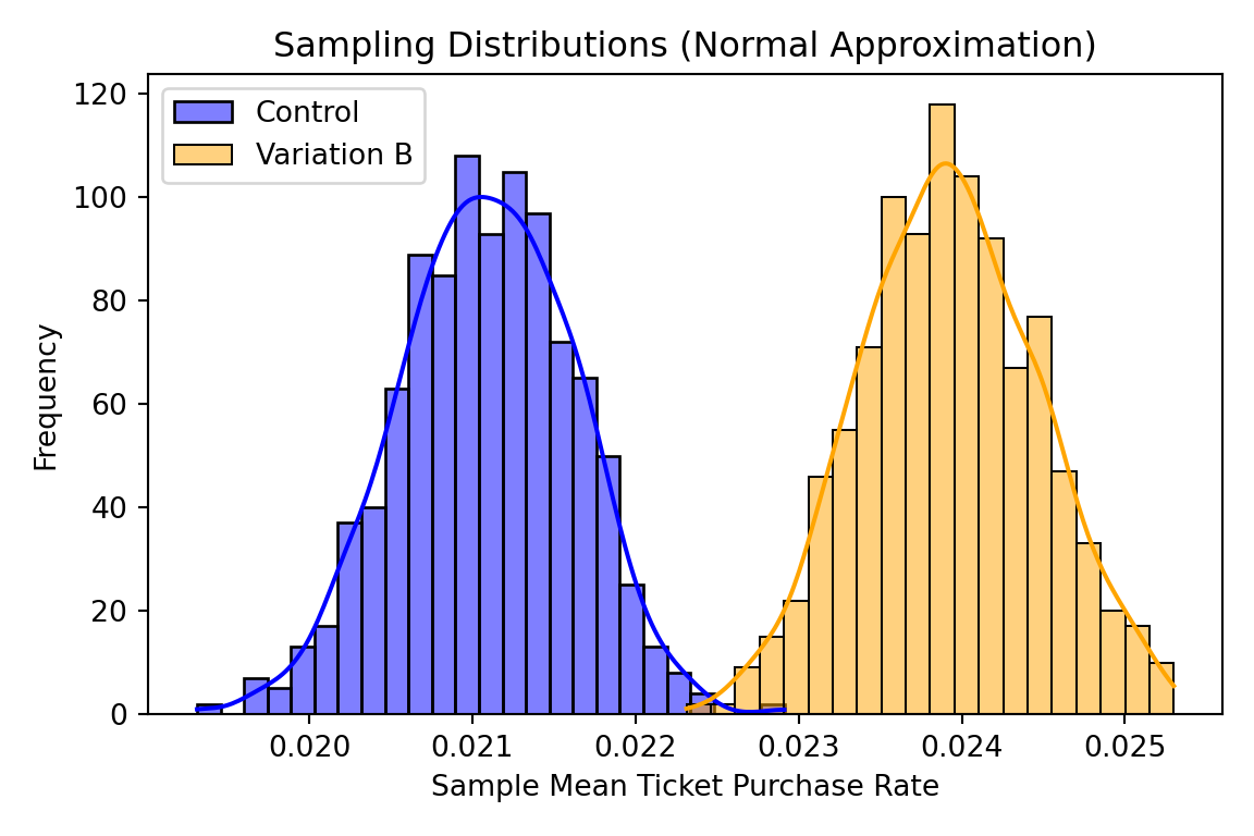

## Control group size: 85000
## Variation B group size: 85000
## Number of random samples generated for each group: 1000
## Size of each random sample: 80000

If we take fairly large sample sizes and enough samples we can see that these two distributions are distinct and our test tells us the results are likely significant and reproducible.

Recommendation

We can recommend variation_B as statistically significant, at the 95% confidence level, if the Confidence Interval for the difference represents a reasonable lift for our investment. We might argue, that unless the lower end estimate we calculated of 0.14% would produce enough revenue to pay for the development, building it may not return the investment.

A/B/N Testing in Python