Libraries Used

library(tidyverse)
library(readr)
library(ggplot2)
library(caret)
library(knitr)
library(quanteda)
library(doSNOW)
library(gridExtra)
library(quanteda.textplots)

In the first part we trained a single decision tree with our document-frequency matrix using just the tokenized text. i.e. simple Bag-of-words approach. Now let’s see if I can use some n-grams to add some word order element to our approach to see if we get better results. The one caveat is that creating n-grams explodes our feature space quite significantly. Even a modest approach leads to tens-of-thousands of features and a very sparse feature matrix. Also, since I are doing this on a small laptop this quickly grows into something unwieldy. Therefore I will not go through the interim step of building a similar single decision tree model with this larger feature matrix. Instead I will use a technique to reduce this feature space down to a manageable level. I’ll use Singular Value Decomposition to achieve this.

## Warning: remove_twitter, remove_hyphens arguments are not used.

TF-IDF

So let’s create a term-frequency inverse frequency matrix to train on. This adds some weight to the words that make up the term in a document. Instead of a count of the number of times a word appears in a document we get a proportion.

train_tfidf <- dfm_tfidf(train_dfm, scheme_tf = 'prop')

Check if we have any incomplete cases.

which(!complete.cases(as.matrix(train_tfidf)))

## integer(0)

Good we have none. Now create a dataframe and clean up any problematic token names we might have as a precaution.

train_tfidf_df <- cbind(Sentiment = train$Sentiment, data.frame(train_tfidf))
names(train_tfidf_df) <- make.names(names(train_tfidf_df))

N-Grams

We can use the below method to create any number of N-grams or combinations of works. Let’s create some bigrams and see if this will improve our score. This will make our feature space very wide and be quite computationally expensive. In order to run this on a small laptop we will need to do some dimensionality reduction before trying to run any models with these bigrams. Later we may try some skip-grams as well.

train_tokens <- tokens_ngrams(train_tokens, n = c(1,2))
train_tokens[[2]]

##  [1] "think"          "felt"           "realli"         "sick"          
##  [5] "depress"        "school"         "today"          "cuz"           
##  [9] "stress"         "glad"           "got"            "chest"         
## [13] "think_felt"     "felt_realli"    "realli_sick"    "sick_depress"  
## [17] "depress_school" "school_today"   "today_cuz"      "cuz_stress"    
## [21] "stress_glad"    "glad_got"       "got_chest"

Taking a look at a few terms we have created.

train_tokens[[4]]

## [1] "hug"                "@ignorantsheep"     "hug_@ignorantsheep"

Now coverting to a matrix.

train_matrix <- as.matrix(train_dfm)
train_dfm

## Document-feature matrix of: 4,732 documents, 9,581 features (99.92% sparse) and 0 docvars.
##        features
## docs    case feel emo camp wee bit alr bring human right
##   text1    1    2   1    1   1   1   1     1     1     1
##   text2    0    0   0    0   0   0   0     0     0     0
##   text3    0    0   0    0   0   0   0     0     0     0
##   text4    0    0   0    0   0   0   0     0     0     0
##   text5    0    0   0    0   0   0   0     0     0     0
##   text6    0    0   0    0   0   0   0     0     0     0
## [ reached max_ndoc ... 4,726 more documents, reached max_nfeat ... 9,571 more features ]

A quick peak at the wordcloud.

# Create wordcloud
train_dfm %>% textplot_wordcloud()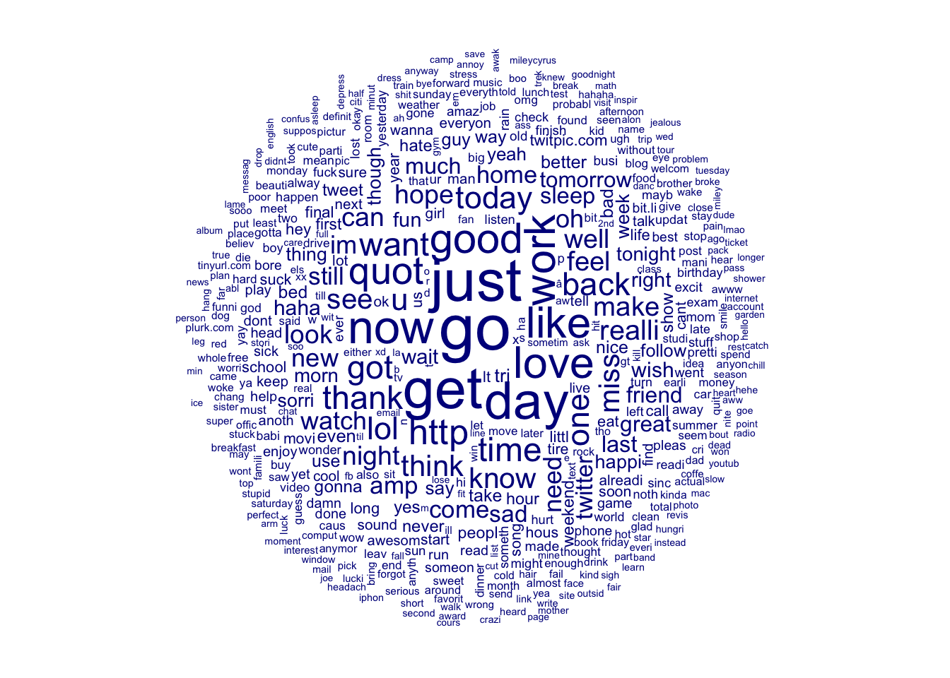

Converting the train_dfm to a matrix so that we can column-bind it to the Sentiment scores as a dataframe.

# Convert to matrix
train_dfm <- as.matrix(train_dfm)

# Bind the DFM, Sentiment together as a dataframe
train_df <- cbind("Sentiment" = as.factor(train$Sentiment), 
                  as.data.frame(train_dfm))

Again make sure names are clean.

# Alter any names that don't work as columns
names(train_df) <- make.names(names(train_df), 
                              unique = TRUE)

Garbage collection.

gc()

##             used   (Mb) gc trigger   (Mb) limit (Mb)  max used   (Mb)
## Ncells   2814476  150.4    4348530  232.3         NA   4348530  232.3
## Vcells 187569119 1431.1  298873490 2280.3      32768 207428674 1582.6

Set up our Multifolds and train control for 30 partitions.

# Set seed
set.seed(42)
# Define indexes for the training control 
cv_folds <- createMultiFolds(train$Sentiment, 
                             k = 10, times = 3)
# Build training control object
cv_cntrl <- trainControl(method = "repeatedcv", 
                         number = 10,
                         repeats = 3, 
                         index = cv_folds)

# Train a decision tree model using 
# the training control we setup
#start.time <- Sys.time()

# Create a cluster to work on 10 logical cores.
#cl <- makeCluster(3, type = "SOCK")
#registerDoSNOW(cl)

# rpart2 <- train(Sentiment ~ ., 
#                 data = train_df, 
#                 method = "rpart", 
#                 trControl = cv_cntrl, 
#                 tuneLength = 7)
 
 # Processing is done, stop cluster.
#stopCluster(cl)

# Total time of execution on workstation was 
#total.time <- Sys.time() - start.time
#total.time

Use the irlba package for Sigular Value Decomposition

library(irlba)

## Loading required package: Matrix

## 
## Attaching package: 'Matrix'

## The following objects are masked from 'package:tidyr':
## 
##     expand, pack, unpack

train_tfidf

## Document-feature matrix of: 4,732 documents, 9,581 features (99.92% sparse) and 0 docvars.
##        features
## docs         case      feel       emo      camp       wee       bit       alr
##   text1 0.1750632 0.1821106 0.1881131 0.1526979 0.1984715 0.1301557 0.2161791
##   text2 0         0         0         0         0         0         0        
##   text3 0         0         0         0         0         0         0        
##   text4 0         0         0         0         0         0         0        
##   text5 0         0         0         0         0         0         0        
##   text6 0         0         0         0         0         0         0        
##        features
## docs        bring     human     right
##   text1 0.1437998 0.1984715 0.1015091
##   text2 0         0         0        
##   text3 0         0         0        
##   text4 0         0         0        
##   text5 0         0         0        
##   text6 0         0         0        
## [ reached max_ndoc ... 4,726 more documents, reached max_nfeat ... 9,571 more features ]

Create our reduced feature space.

# Time the code execution
start.time <- Sys.time()

# Perform SVD. Specifically, reduce dimensionality down to 300 columns
# for our latent semantic analysis (LSA).
train.irlba <- irlba(t(as.matrix(train_tfidf)), nv = 300, maxit = 600)

# Total time of execution on workstation was 
total.time <- Sys.time() - start.time
total.time

## Time difference of 2.755332 mins

Create a new dataframe with the reduced feature space.

train.svd <- data.frame(Sentiment = train$Sentiment, train.irlba$v)

Train a random forrest model and see if our results improve.

# Create a cluster
cl <- makeCluster(4, type = "SOCK")
 registerDoSNOW(cl)

# Time the code execution
start.time <- Sys.time()

rf.cv.4 <- train(Sentiment ~ ., data = train.svd, method = "rf", 
                 trControl = cv_cntrl, tuneLength = 4)

# Stop cluster.
stopCluster(cl)

# Total time 
total.time <- Sys.time() - start.time
total.time

load(file = "../../rf1.rds")
rf.cv.1

## Random Forest 
## 
## 4732 samples
##  500 predictor
##    2 classes: 'Negative', 'Positive' 
## 
## No pre-processing
## Resampling: Cross-Validated (10 fold, repeated 3 times) 
## Summary of sample sizes: 4258, 4258, 4259, 4259, 4259, 4260, ... 
## Resampling results across tuning parameters:
## 
##   mtry  Accuracy   Kappa    
##     2   0.6647551  0.3295559
##    12   0.6767312  0.3535059
##    79   0.6799018  0.3598693
##   500   0.6732108  0.3465657
## 
## Accuracy was used to select the optimal model using the largest value.
## The final value used for the model was mtry = 79.

Outputting the model results we see that we have an accuracy of 68% accuracy. This is still not great. We can’t expect to get very high accuracy with this data. Tweets is especially ripe with scarcasm and other problems that makes sentiment analysis difficult. I was hoping for 80%-90% accuracy, but this may not be possible with decision trees. We can try some other feature engineering techniques, but it is unlikely we will improve much more without some sort of breakthrough.

Combine Skipgrams with N-grams

The next thing we can try is using skipgrams or maybe a combination of skip-grams and n-grams. Here is an example of skip grams.

train_tokens2 <- tokens_skipgrams(train_tokens, n = 2, skip = 1)
train_tokens2[[2]]

##  [1] "think_realli"               "felt_sick"                 
##  [3] "realli_depress"             "sick_school"               
##  [5] "depress_today"              "school_cuz"                
##  [7] "today_stress"               "cuz_glad"                  
##  [9] "stress_got"                 "glad_chest"                
## [11] "got_think_felt"             "chest_felt_realli"         
## [13] "think_felt_realli_sick"     "felt_realli_sick_depress"  
## [15] "realli_sick_depress_school" "sick_depress_school_today" 
## [17] "depress_school_today_cuz"   "school_today_cuz_stress"   
## [19] "today_cuz_stress_glad"      "cuz_stress_glad_got"       
## [21] "stress_glad_got_chest"